VLOOKUP Troubleshooting in Google Sheets
Using the VLOOKUP function is a fast and easy way to find information in Google Sheets when the data is organized in columns. It is however easy to make a mistake while writing a VLOOKUP formula. This page describes the most frequent errors you could face and how to troubleshoot them.
#N/A error

Did not find value "__" in VLOOKUP evaluation
There is a typo in the Lookup value
Typos are a simple and common reason. Check that the Lookup value is spelled correctly. Typos can also generate the Wrong number of arguments error message. In that case, make sure no separators are missing between the parameters.
Approximate match is incorrectly configured
If the VLOOKUP function searches for the value closest to and inferior to the value you are looking for. The #N/A error can appear in two cases:
- The lookup value is smaller than the smallest value in the lookup array.
- The lookup column is not sorted in ascending order.
For more information, see approximate match.
The Lookup value doesn't exist
If you are searching for an exact match (FALSE), and the Lookup value doesn't exist in the first column of the Search range, #N/A will be returned.
For more information, see exact match.
You can replace N/A results with an empty or user-friendly value with the IFNA formula.
Wrong data format
The format of the Lookup value must match the format of the matching value in the Search range. In particular, make sure that numbers are formatted the same way, as numbers, and not text.
Hidden spaces or non-printing characters
There may be extra spaces in your Lookup value. You can use the TRIM function to remove hidden spaces. For example =VLOOKUP(TRIM(G4), B7:D12, 3, FALSE).
Results spill over to non-empty cells
This can happen if you use VLOOKUP with arrays and return multiple results. Make sure that there are enough empty cells below and next to the formula's cell.
A value is not available to the formula or function
Path to the Search range is not provided
This error occurs if VLOOKUP is not able to find the Search range.
- Check for typo in the Search range
- If the Search range is in a different sheet of the Lookup value, you must specify the sheet's name followed by the exclamation mark. For example, if the Search range B4:D7 is located in a sheet namedSheet2, the parameter is
Sheet2!B4:D7 - If the Search range is in a different spreadsheet, the Search range must include the IMPORTRANGE function with the URL of the spreadsheet and specify the sheet's name followed by the exclamation mark.
For example, if the Search range is located in a spreadsheet named Data range, and in a sheet named Sheet1, the parameter isIMPORTRANGE("https://docs.google.co[...]","Sheet1!B4:D7")
For more information, see how to use VLOOKUP from another sheet.
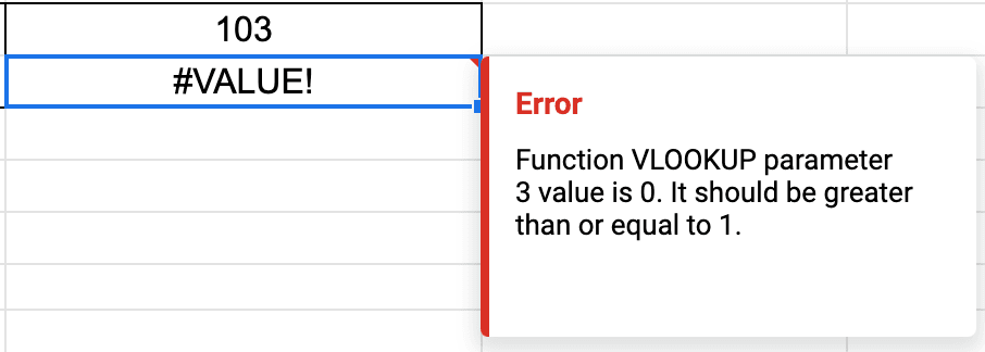
#VALUE! error

Function VLOOKUP parameter 3 is 0. It should be greater than or equal to 1
The Column number is not found
Make sure that the Column number is at least 1. The reason is that column indexing of a range starts at 1.
An array value could not be found
A VLOOKUP parameter is missing
Check if a parameter is missing within the VLOOKUP function. VLOOKUP works with a minimum of three parameters (the Lookup value, Search range, and Column number are required).
#REF! error

VLOOKUP evaluates to an out of bounds range
The Column number is greater than expected
Make sure the Column number you specified isn’t greater than the number of columns in the Search range.
For example, if the Search Range is B7:D9, the Column number can be either 1 (column B), 2 (column C), or 3 (column D).
Unresolved sheet name "__"
Path to the Search range is incorrect
You'll get this error if the Search range is in a different sheet and VLOOKUP cannot find the sheet's name you provided. Make sure to specify the correct path.
For more information, see how to use VLOOKUP from another sheet.
#NAME? error

Unknown function
Typo in the function name
If you get the #NAME error, Google Sheets cannot interpret the VLOOKUP function. It's probably because there is a typo in the function name.
Unknown range name: '__'
Can't find the range
The #NAME error can appear because VLOOKUP thinks you named a range. Make sure to add quotation marks around it.
#ERROR! error

Formula parse error
Usually a parenthesis problem
This error means that Google Sheets can't interpret your formula, most of the time due to incorrect use of parentheses. Make sure you close each open parenthesis in the right place, and have the same number of opening and closing parenthesis.
For more information, see how to use VLOOKUP.
General VLOOKUP tips
- The Lookup value must be in the first column of the Search range
- The format of the Lookup value must match the format of the matching value in the Search range
- Make sure there is no hidden space or apostrophes in the first column of the Search range
- If you are using text in the formula, add quotation marks around that text
- Add commas between each parameter
- If you drag down the formula, lock the search range (with $)
- Add the name of the sheet followed by an exclamation mark if the Search range is referenced in another sheet
- Make sure to point to the correct column in the Search range
- Use the correct Approximate match parameter value
- If you use TRUE as an approximate match (or don't specify one), make sure the values in the first column of the Search range are sorted in ascending order
- If you use FALSE as an approximate match, make sure the Lookup value is in the first column of the Search range